Breaking Down Abstractions: Database Indexes
July 23, 2018 · Filed in Breaking AbstractionsIn the introduction to this blog, I mentioned that I love breaking down abstractions to understand what makes them tick. This blog post is the first of many that will break down a fascinating abstraction.
Abstraction
Database indexes provide the abstraction of performant queries with the cost of some overhead during writes and additional storage space. As most workflows are read-heavy, the overhead of indexes is almost always worthwhile.
Indexes are incredibly powerful. The difference between a query that can utilize one or more indexes and a query without indexes can be breathtaking on datasets larger than a few hundred objects. In fact, the difference can be that the query with indexes finishes in milliseconds while the index-less query causes the database to fall over!
I mentored an intern through a project with a database component last summer. Once the database grew to a substantial size, he remarked that his queries were taking seconds to complete, which was much longer than on his test dataset of a few items. I questioned whether indexes were in place and had him tack on EXPLAIN to the start of his query (most databases, SQL or NoSQL, have some notion of EXPLAIN which details the steps in executing the given query). While he did have some indexes, it was evident from the results of the EXPLAIN that none of them were being used; rather the entire database was being scanned (known as a full table scan). We identified and added the missing index. The query wasn’t just twice as fast, it was two orders of magnitude faster, so about 10 milliseconds. I think his reaction may resonate with some of you: “Clearly I need to learn more about indexes.”
Why do the right indexes lead to potentially massive performance increases? Conversely, why can the wrong index cause slow queries or even the database to fail? Why are indexes so important? Let’s break down this abstraction.
Breaking it down
To understand how database indexes work under the hood, let’s define a simple table which lists several people, their ages, and associated IDs:
| id | name | age |
|---|---|---|
| 1 | Arvilla Hawks | 24 |
| 2 | Maryellen Gourd | 18 |
| 6 | Corliss Henline | 38 |
| 8 | Lidia Haught | 17 |
| 9 | Leo Thurlow | 84 |
| 14 | Raymundo Vavra | 23 |
| 26 | Lyn Stucky | 28 |
| 28 | Lura Apodaca | 11 |
| 30 | Brook Milum | 81 |
Given an ID, we’d like to find out the name and age. Here’s a SQL query to discover that Leo Thurlow (age 84) is stored at ID 9:
SELECT name, age FROM people WHERE id = 9How does this query find the right answer? Well, without indexes, it merely scans the rows of the table until it happens upon ID 9. This ID was just a few entries from the start, so that doesn’t sound too bad. Consider, however, that this table could be thousands, millions, or billions of rows long. What if ID 9 was the last row? We’d have to scan through a lot of rows! This process of scanning each row has a time complexity of O(N). Not great.
It’s also worth noting that if the id column was not unique, it would become necessary to scan all entries to find all the ones with the given ID. When N is large, scanning N items every time we need to respond to a query is going to take a long time. It’s possible that a long-running query combined with lots of other concurrent queries could just cause a database to fail (it could run out of memory, go into swap, become unable to respond to healthchecks, and be removed from the cluster).
What we need is some way to store the IDs in a data structure more suited to this kind of searching. Enter: the index!
Indexes are used to quickly locate data without having to search every row in a database table every time a database table is accessed. Indexes can be created using one or more columns of a database table, providing the basis for both rapid random lookups and efficient access of ordered records.1
There are many different types of database indexes, including B-tree, R-tree, Hash, Bitmap, and Spacial. Rather than trying to cover all of these index types, let’s deep dive on the ubiquitous B-tree.
Binary Search Tree vs. B-Tree vs. B+ Tree
Many software engineers are understandably confused about the differences between these three very similar sounding data structures: binary search tree, B-tree, and B+ tree. While they are all tree data structures, they are not synonymous. A B-tree is not a “binary” tree (no matter how convenient that would be)! In fact: “What, if anything, the B stands for has never been established.”2
Binary Search Tree
Binary search trees are binary trees that keep their keys in sorted order by enforcing the requirement that all left children of a node have values less than the node’s and all right children have values greater than the node’s.

B-tree
B-tree is a self-balancing tree data structure that keeps data sorted and allows searches, sequential access, insertions, and deletions in logarithmic time. The B-tree is a generalization of a binary search tree in that a node can have more than two children.2

B-trees have these properties:
- Can have more than two children
- Self-balancing
- Internal (non-leaf) nodes may be joined or split in order to maintain balance
- All leaf nodes must be at the same depth
- The number of children for a particular node is equal to the number of keys in it plus one
- The minimum and maximum number of child nodes are typically fixed (a 2-3 B-tree allows each internal node to have 2 or 3 child nodes)
- Minimizes wasted storage space by ensuring the interior nodes are at least half full
In our simple B-tree, we store only a few keys in each node and each node only has a small number of children. A practical B-tree would have far more keys and children–the exact number is related to the size of a full disk block such that each read will get as much data as possible.
To use a B-tree as a database index, we must either store the entire table rows or hold pointers to the rows. Let’s take the pointer approach:
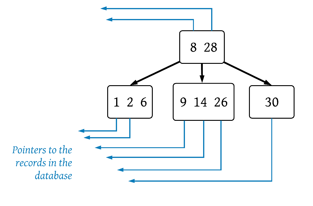
Note that this B-tree has the properties outlined above:
- All leaf nodes are at the same depth
- The
[8 28]node has two keys and therefore three children - Values less than 8 are in the left subtree, values between 8 and 28 and in the middle subtree, and values greater than 28 are in the right subtree
- Wasted space is minimized and the tree is balanced
Let’s return to the people table we started with and rerun the query now that we have an index structure in place. When evaluating the WHERE clause (WHERE id = 9), the query optimizer now sees there is an index on the id column. It follows the B-tree data structure until it finds ID 9 and follows the pointer to the associated table row.
- Is 9 equal to 8? No
- Is 9 less than or equal to 8? No
- Is 9 between 8 and 28 (inclusive)? Yes!
- Is 9 equal to 9? Yes!
- Which table row does 9 point to?
9 | Leo Thurlow | 84
The time complexity for this search drops from O(N) to O(log(N))!
B+ tree
A B+ tree is an N-ary tree with a variable but often large number of children per node. … A B+ tree can be viewed as a B-tree in which each node contains only keys (not key–value pairs), and to which an additional level is added at the bottom with linked leaves.3
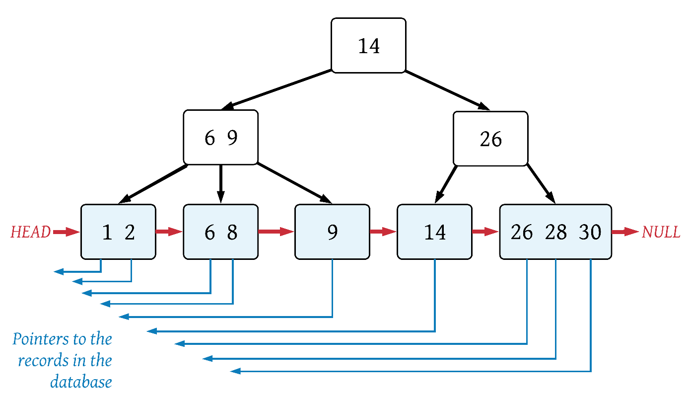
B+ trees have these additional properties relative to a B-tree:
- Leaf nodes are linked together
- All keys (and pointers to table rows) are stored in the leaves
- Copies of the keys are stored in the internal (non-leaf) nodes
- Typically have a large number of children per node
- Each node may store a pointer to the next node for faster sequential access
Comparing the example B-tree and B+ tree reveals that the same data is stored in each, but the additional properties of the B+ tree force the keys down to the leaf nodes. The linked list this forms makes range queries more efficient.
Progression
Given those definitions, it becomes clear that each of these tree data structures builds on the previous one in a progression towards a structure fit for a database index. The added complexity with each step is a trade-off for improved performance in particular use cases. Some databases use a combination of B-trees and B+ trees depending on the type of index and nature of queries.
Here is one way of looking at the progression from binary tree to B+ tree:
- Start with a simple binary tree. Add self-balancing and enforce the properties of a binary search tree. Result: balanced binary search tree
- Allow this balanced binary search tree to have more than two children and enforce other properties of a B-tree. Result: B-tree
- Add pointers from the stored keys to rows in the database table. Result: B-tree used as a database index
- Push all keys into the leaf nodes and link the leaves. Result: B+ tree used as a database index
Further reading
- Wikipedia: Database Index
- Wikipedia: B-Tree
- Wikipedia: B+ Tree
- JavaScript B-Tree Demo
- B+ Tree Visualization
- Straightforward B+ Tree Implementation in JavaScript
- Comparison of B-Tree and Hash Indexes
Metadata and Navigation
Subscribe
Subscribe via my newsletter or RSS feed